Can a 30B Local LLM Run on a MacBook? 1.58-Bit Ternary Quantization

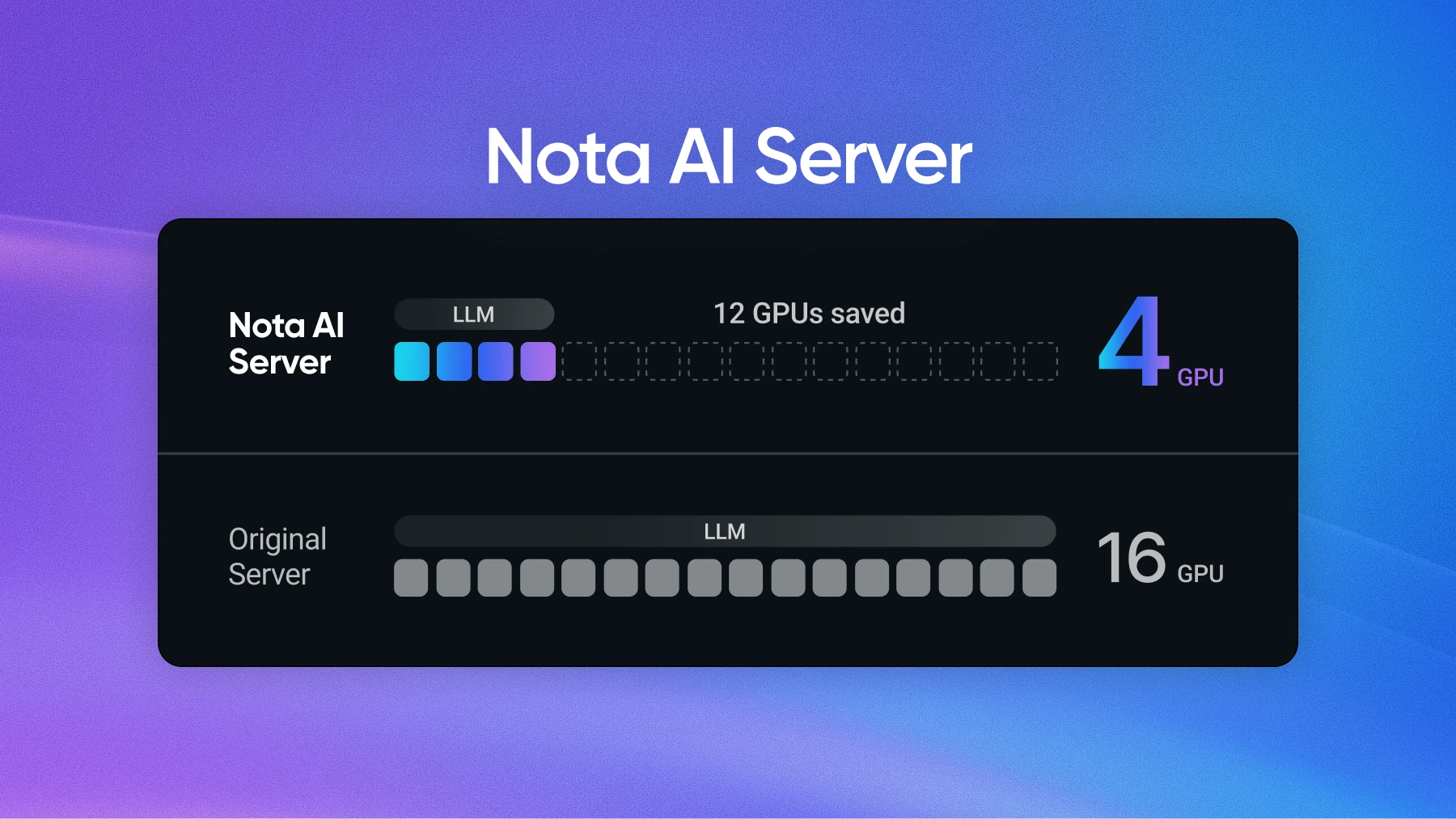
In LLM quantization, the practical floor is often put at 4 bits. Going below that shrinks the file but sharply lowers answer quality. For local LLMs, this constraint is even tighter.

For complex coding or multi-step tasks, people usually consider 27B–30B models the practical starting point. But even at 4 bits, a 30B model's weights alone are around 16GB. Add runtime memory and the KV cache, and it will not fit on a 16GB machine and is tight even on a 24GB MacBook.

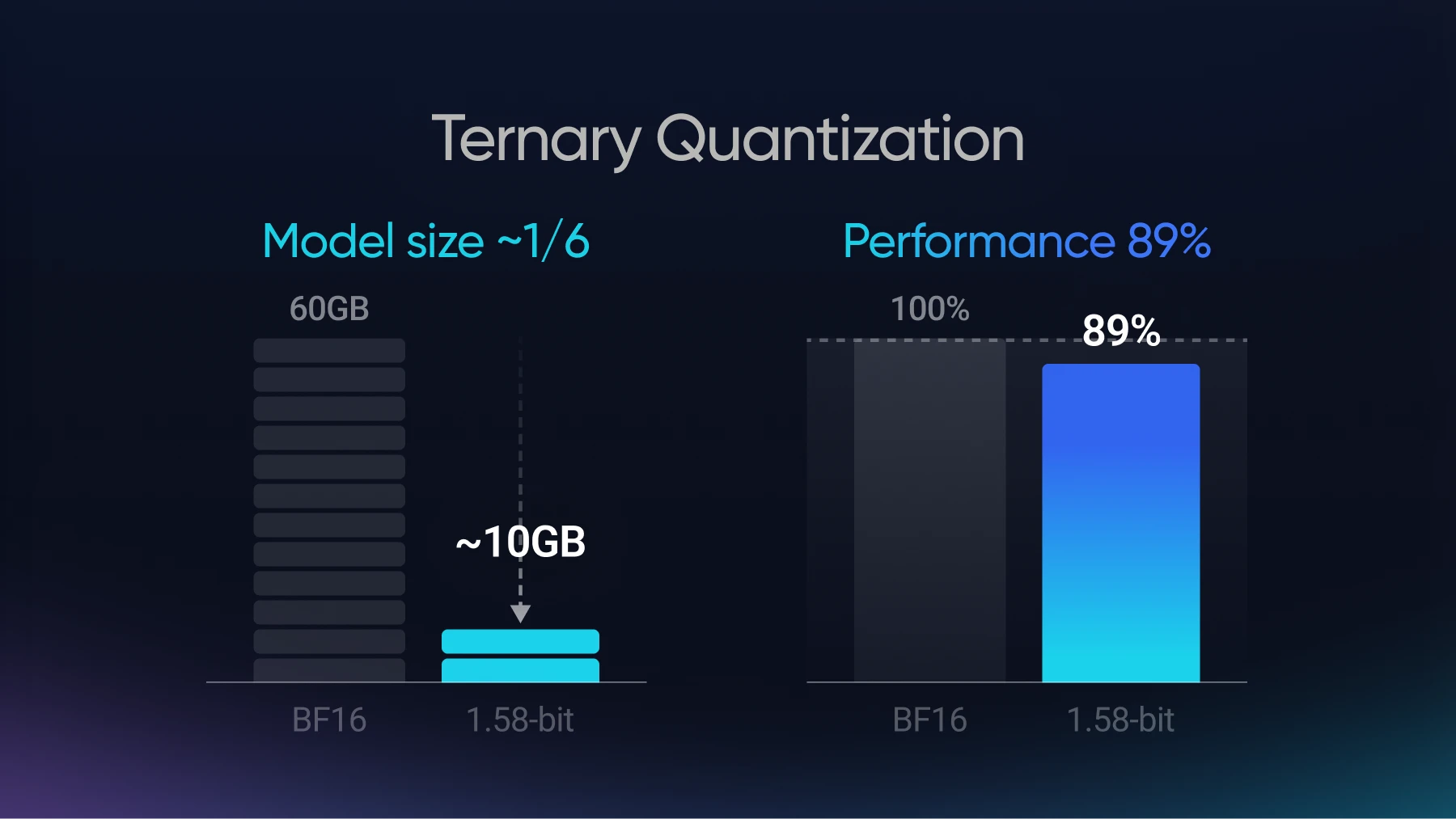
So Nota AI kept the model size at 30B and pushed the bits below 4. The method is 1.58-bit quantization, which represents the weights of NVIDIA's Nemotron 3.5 Lightning 30B (A3B) with only three values: -1, 0, +1. The model shrank to about 10GB, and performance recovered to about 89% of the original on the generative benchmark average. This post walks through that process.

What Is 1.58-Bit Quantization?

1.58-bit quantization is ternary quantization that represents an LLM's weights with only three values: -1, 0, +1. It is called 1.58-bit because the theoretical minimum number of bits needed to distinguish three values is log₂3 ≈ 1.585 bits. Here, 1.58-bit refers not to the file size stored on disk but to the amount of information one value carries. A real file also stores a scale factor alongside the weights, so the bits per parameter come out higher than this.

Once converted to ternary, each entry of the weight matrix becomes one of -1, 0, +1 depending on its magnitude and sign. Small values near zero become 0, and the rest keep only their sign.

There are two main paths to a 1.58-bit model.

• QAT (Quantization-Aware Training): like BitNet b1.58, start from random initialization and pretrain with the weights fixed to ternary from the start.
• PTQ (Post-Training Quantization): take an already-trained BF16 checkpoint and convert it to ternary afterward.

For this work, we chose PTQ, because it lets us reuse an already-trained model instead of redoing pretraining from scratch.

How Ternary Quantization Works

Ternary quantization has three steps. In the end, two things need to be set: below which magnitude a weight counts as 0 (the threshold τ), and to what magnitude the remaining weights are reconstructed (the scale s). The figure below lays out the key formula for each step.

To make this concrete, let's follow the calculation on an example group of eight weights. For this group, α is 0.39, the threshold τ is 0.195, and the reconstruction scale s is 0.58. The figure below shows how each weight turns into a ternary code and a reconstructed value.

What matters here is the share of weights that become 0. If too few become 0, even small values near zero grow to ±1 and the reconstruction error increases; if too many, less information remains and the model's expressiveness drops. The threshold τ sets this share, and in the example group three of the eight became 0.

Why It Scores Zero As-Is

PTQ by the procedure above finished without a hitch. But in our internal evaluation, GSM8K and HumanEval came out at 0.00, and IFEval-ko, which measures Korean instruction-following, at 10.36.

The direct cause is rounding error. As in the earlier example where 0.90 becomes 0.58 after reconstruction, each weight picks up a reconstruction error, and this error accumulates layer by layer. In a structure like a transformer, which stacks dozens of layers to predict the next token, the per-layer error feeds into the final output probabilities, and on generative benchmarks, where the model must produce its answer token by token, this means it almost never gets the right answer.

In fact, this is common in extreme low-bit quantization at 2 bits or below. It is the same reason the introduction put 4 bits as the practical floor for LLM quantization. Shrinking the file by lowering the bit count and keeping the model's ability are separate problems, and the lower the bit count, the wider that gap.

So how do you bring a zero-scoring model back? We approached it in two steps.

Recovery Step 1: On/Off-Policy Distillation

The first technique is distillation. The common choice is off-policy distillation, where the student follows answers the teacher generated in advance. On its own, though, the outputs the student actually produces, already distorted by quantization, barely show up in the training signal, and in a ternary model, whose output distribution shifts a lot after quantization, that gap grows larger. So this time we applied on-policy distillation alongside off-policy distillation.

Here, on-policy means the student learns from context it generated itself. When the student (the ternary model) generates answer tokens, the BF16 teacher computes the probability distribution of the next token in that same context. The student receives the difference between the teacher's distribution and its own as a learning signal. By analogy, the teacher follows the student's written solution line by line and, at each line, points out "here is what I would have written next." Applying on-policy was also about pulling the output distribution, shifted by quantization, back toward the teacher.

The remaining problem is that quantized weights cannot be differentiated. For this we use the STE (Straight-Through Estimator). In the forward pass it uses the ternary code as-is, and in the backward pass it treats the quantization function as an identity function and passes the gradient to the latent weights. Latent weights are the full-precision values kept behind the ternary code; as small updates accumulate they shift gradually, and the moment one crosses the threshold τ, its quantized code flips.

Because of this structure, the weights whose code actually changed over one epoch (one pass through the full training data) were about 5–7% of the total. This means recovery is less about putting new knowledge into the model and more about fixing the small number of codes that quantization changed so they match the original output. In fact, when we ask the recovered model to introduce itself in Korean, it answers that it is Nemotron, built by NVIDIA researchers. This is an indirect sign that the original model's identity stayed intact through recovery.

Recovery Step 2: Boundary Masking

Distillation and STE alone push performance up sharply within the first one or two epochs. Across epochs 1 and 2, GSM8K rose to 82.56 then 87.57, HumanEval to 72.56 then 80.49, and IFEval-ko to 61.79 then 68.39.

But adding more epochs did not keep performance rising. Training to 3 epochs under the same conditions sent GSM8K back down to 85.90 and IFEval-ko to 64.82. The same pattern showed up when we repeated the experiment with other models. It looked like STE, by passing a signal to every latent weight, kept updating even values that did not need to change, so noise was flipping codes. So we narrowed the range of weights to train.

We trained only the weights whose PTQ initial value sat within ±10% of the threshold τ, about 5.9% of the total, and froze the rest of the latent weights. We narrowed it to the boundary region because only weights in that range can actually flip their code with a small update. Values far from the boundary rarely change code even with training and can only add noise. We call this approach boundary masking.

Applying boundary masking at the same 3 epochs brings GSM8K back up from 85.90 to 88.32 and IFEval-ko from 64.82 to 68.39. In other words, deciding where to train mattered more than training longer.

Results: 89.4% on the Generative Benchmark Average

The recovered model scored 83.82 against the original's 93.80 on the seven-benchmark generative average, 89.4% of the original. GSM8K, which was 0.00 right after the post-training conversion, recovered to 89.31, about 94% of the original.

By benchmark, math (GSM8K) and code (HumanEval) reached about 94% of the original, and five of the seven were at or above 89% of the original. The lower-recovery items were MATH500, which requires long solutions, and Korean instruction-following (IFEval-ko), which are areas to improve further.

Running It on a MacBook

So how much memory does a MacBook need to run this model? On a Mac, the GPU does not use all of the unified memory; by default it uses only about two-thirds to three-quarters. Calculating conservatively at two-thirds, the GPU limit is about 10.7GB on a 16GB MacBook and about 16GB on a 24GB MacBook.

The model's weights are about 10GB, but running it also needs the KV cache, the Mamba state, and runtime buffers. Nemotron 3.5 Lightning is a hybrid architecture that uses Mamba layers and Attention layers together, and because only six Attention layers need a KV cache, the KV cache takes about 0.8GB even at a 128K-token context. Calculated from the public config file, memory beyond the weights is at most about 2.4GB, and the total at most about 12.4GB. That is larger than the limit on a 16GB MacBook and smaller than the limit on a 24GB MacBook.

A 16GB MacBook can also fit it on paper if you raise the GPU memory limit in macOS settings, but that sharply cuts the memory left for the system and other apps. So we recommend a MacBook with 24GB or more.

The model is available on Hugging Face, so you can download it from the repository below and run it yourself. The model released now is a preview checkpoint whose performance recovery is still ongoing, and the model card lays out the storage format and evaluation setup.