Tech
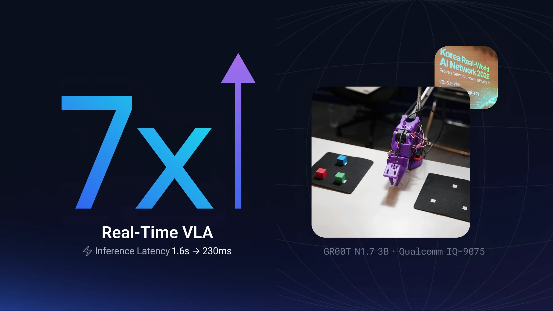
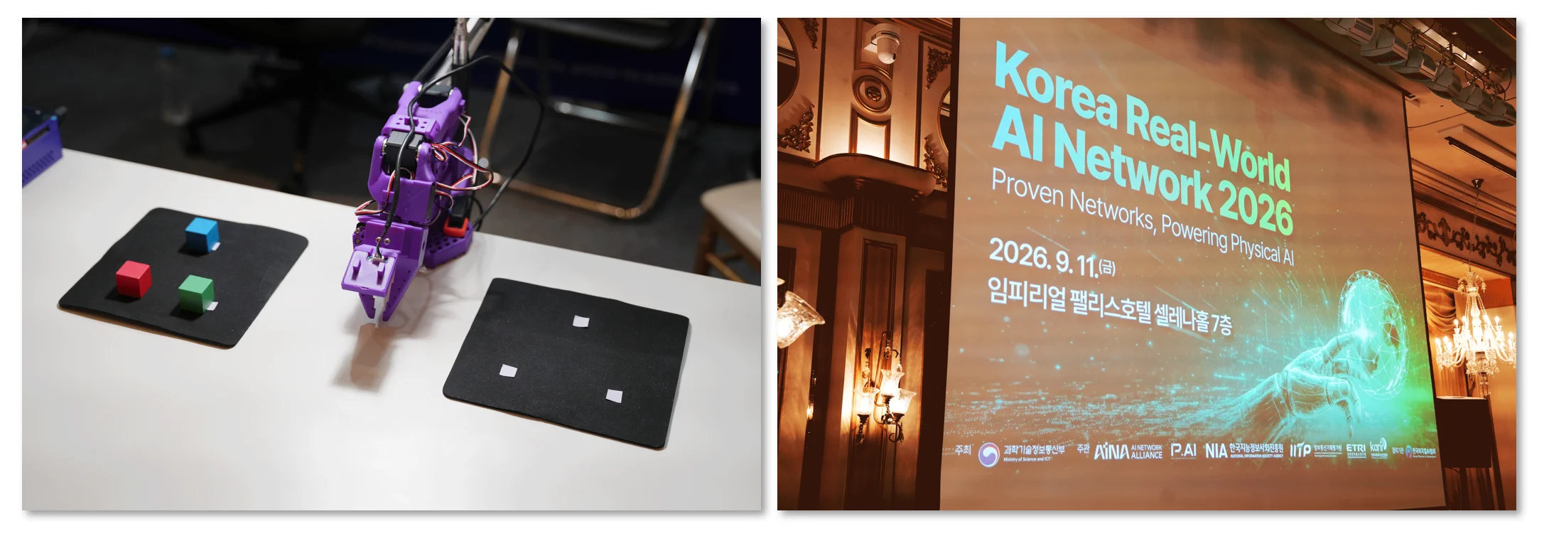
On September 11, KRAIN 2026 (Korea Real-World AI Network) opened in Seoul. It was a place where proof-of-concept cases in AI networks and Physical AI came together, and Nota AI ran a live demo of an SO-101 robot arm driven by a VLA model. On a mat holding cubes of several colors, when a visitor picked one color, the robot picked up only that color and moved it to the other side. This arm ran not on a GPU server but on an NPU on a palm-sized board (Qualcomm Dragonwing IQ-9075).
VLA (Vision-Language-Action) is a model that takes camera frames and natural-language instructions together and outputs robot actions. It is a leading branch of robotics foundation models (RFM). One model handles seeing, deciding, and putting out the next motion. Because it recomputes this entire process on every frame, running it in real time within the limited resources of an NPU is itself the bottleneck. This article lays out the five decisions we faced while solving that bottleneck.
For a battery-powered robot, the power the computation draws is operating time, and the heat it makes is fans and bulk. In mass production, where hundreds of units must be deployed, the price of the brain board decides whether the business works. That is why the slot goes to an NPU SoC, designed for compute-per-watt efficiency and integrating control, vision, and communication on one chip. Qualcomm recently released a 700-TOPS-class robotics SoC with a multi-core NPU, and Intel declared it would replace the GPU in the robot brain. Both point the same way.
This constraint does not spare any form factor. Humanoids have many joints and carry their own battery, so their power and thermal budgets are tight. But wheeled autonomous mobile robots (AMRs), which get deployed widely in the field, and fixed robot arms also struggle to carry a whole GPU module. It means the VLA developed and demonstrated in the GPU ecosystem eventually has to move onto an edge NPU. That is why the KRAIN demo targeted the Hexagon NPU of the Qualcomm IQ-9075.
But there is no model you can pick up and deploy right away. As LLM progress did, the RFM field is now focused on accuracy and generality rather than inference efficiency. There is still no open-source model that works out of the box in any environment and on any robot, so fine-tuning per environment is mandatory. Models aimed at lightweight deployment, like SmolVLA, are starting to appear, but if the model market is at an early stage, the optimization of those models is at an even earlier one.
There is also almost no literature on how to move them. Since most research assumes GPU compute, the latency that gets published is on an H100 basis. Papers on the methodology are hard to find, and the most you will find are tutorials a chip vendor put out for a few specific models. How many times slower the same model runs on an embedded NPU, how far it optimizes, and how much it differs by backbone: there was no way to know short of putting it on the board ourselves.
The joints of the SO-101 used in this demo (a standard 6-DoF robot arm) receive a new target angle 30 times per second (30Hz). That means one step has to come out every 33ms. But a VLA does not emit steps one at a time; it observes once and puts out a whole action chunk (an action plan bundling several steps). GR00T N1.7 is 32 steps and MolmoAct2 is 30 steps, so one chunk is about a second of motion. The time given to one inference is also not 33ms but this one second.
The question is where that one second goes. The default configuration, sync mode, does the next observation and inference only after the chunk is fully used, so inference time is directly the arm's idle time. If inference is one second, it moves for one second and stands still for one second. With camera and robot latency added on top, the bar is set by how much idle time you can tolerate, and that value is set by the robot and the task. Running a 10-step flow matching MolmoAct2 on Jetson Thor, the pick-and-move motion on the cube stayed continuous in the 356–373ms range. We wrapped that range with some margin and set IQ-9075's real-time bar at 320–400ms.
This bar is not only about smoothness. Because the model is trained assuming 30 FPS observation, slower inference does not just make the robot sluggish; it also diverges from the training distribution and can lower the success rate itself.
We chose MolmoAct2 as the first backbone to examine. Its weights are open, so we could control the whole process ourselves, from fine-tuning for the SO-101 arm to rewriting the compute graph. But the conclusion first: we did not use this backbone in the final configuration, because even with optimization pushed to the maximum, it could not reach the target bar.
With the Baseline dropped as-is onto the existing on-device stack, one observe-infer-act cycle (End-to-End, hereafter E2E) on IQ-9075 took 3,681ms. That is nearly ten times over the target bar (320–400ms). From this state we applied optimization at the level of the runtime environment and the compute graph.
The first obstacle in that process was not the model but the runtime environment. One VLA cycle runs three parts in order: Vision Encoder, LLM, and Action Head. But the on-device inference stack is a language-model serving structure that puts one model on one NPU, so there was no way to split these three parts across two NPUs. That means on a two-NPU board, one NPU sat entirely idle. So we built our own runtime: NQRR (Nota QNN Robotics Runtime).
NQRR is Nota AI's own robotics runtime, built to use close to 100% of the resources on the multi-NPU IQ-9075. It splits a VLA's compute graphs across multiple NPUs and runs them in a single process, and we set the operator placement and the data paths by looking at the model structure and the hardware characteristics together. We compared the converted graph's output against the original to confirm the two matched.
On top of that, we left accuracy untouched and changed only the graph and the runtime.
The three techniques cut each module's latency by 30 to 60%, and E2E came down from 3,681ms to 1,173.9ms, a 68% reduction.
1,173.9ms is still close to three times the bar. To see which segment the latency piled up in, we profiled segment by segment in a deployment configuration with the Action Head compressed to one step.
The results: LLM 775.8ms, Vision Encoder 278.5ms, Action Head 136.6ms. Even assuming we fully removed the LLM, the largest share, the Vision Encoder and Action Head alone come to about 415ms. That already exceeds the real-time bar.
What we confirmed here was not a limit of the techniques but a limit of the structure. The LLM segment is a serial chain of small operations with high kernel-launch overhead, like Softmax, Layer Normalization, and Slice, so neither quantization nor pruning works well on it. What does work is shortening the input sequence length, and that is set by the model structure, not the runtime. The remaining option was to change the backbone.
The next question was "which backbone to switch to." The criteria for choosing had already come out of MolmoAct2. The techniques worked; what blocked us was the structure. So we needed a backbone where the same techniques hold structurally. We applied four screening criteria to twelve VLA candidates that could run on the SO-101.
We did not look at accuracy in screening. VLAs require fine-tuning per environment, so accuracy from the literature says nothing about accuracy on the SO-101. So we measured it ourselves. We put five models side by side on IQ-9075 with NQRR and measured directly: GR00T N1.7, VLA-JEPA, X-VLA, and Pi-0.5, which met three or more criteria, plus the baseline MolmoAct2.
We measured accuracy in LIBERO closed-loop simulation, and when we stacked techniques up to just before the success-rate loss crossed 1 percentage point, the speedup multiples were: GR00T N1.7 7.0× (93% → 92%), MolmoAct2 3.8×, X-VLA 2.7×, VLA-JEPA 2.1×, and Pi-0.5 2.1×. Which techniques hold differs by structure, so the gap ran to more than threefold across backbones. This is where the decision to change the backbone mattered more than the decision to add one more technique.
There were two selection criteria: post-optimization latency, and the real-hardware success rate from running the same task with SO-101 fine-tuning attached. The multiple tells you how much faster it gets, but not whether the model actually moves the cube on the SO-101.
The two criteria did not give the same answer. The latency leader was not GR00T, and that backbone had the lowest real-hardware success rate of the five. With both criteria on the table, what remained was GR00T N1.7. Even in the configuration before distillation, it ran at around 400ms on the board, landing at the upper end of the real-time bar, and its real-hardware success rate was 80%. The final backbone was decided here.
With the backbone set, we started again from graph and runtime optimization. GR00T N1.7's Baseline on IQ-9075 was 1,602.4ms. This time the goal was to fit the hardware's characteristics. The reductions below are on an E2E basis.
The three techniques were stacked in sequence on the previous stage's result, and after the three the E2E is 399.0ms. By changing only the graph and the runtime, we reached the upper end of the real-time bar. The configuration that scored 80% in the backbone selection evaluation is this point.
Finally, we applied Step Distillation to reduce the action-chunk generation steps. It is 287.4ms at 2-step, and about 230ms for the latest checkpoint with 1-step distillation (drift) applied. That is about 7× versus the Baseline of 1,602.4ms, comfortably below the real-time bar (320–400ms).
The model was inside the real-time bar, but the arm still stood still for 501ms per cycle, outside it. What remained was in the control loop.
The first was the camera input. While the model took over a second, the roughly 96.5ms wait per frame was buried inside it; once inference dropped below 400ms, that share surfaced on its own. The control loop was waiting synchronously for a frame each time. We separated the camera thread so it constantly refreshes the latest frame into a buffer, and changed the control loop to only reference the buffer. Frame-read time dropped into the 0.1ms range, and as a result arm idle time fell from 501ms to 247ms, and observation latency fell from 700ms to 58ms. We did not change a single line of the model.
The second is jitter at action-chunk boundaries. In sync mode we observed the arm twitching slightly at the moment a chunk switched over. We added temporal smoothing (a reference implementation of a LIPO-family algorithm), and jerk RMS dropped from 5.175 to 0.110 on an open-loop measurement. Whether the success rate held as the motion smoothed out was something to confirm separately in closed loop.
The third is the n_action_steps trade-off. Comparing 16 / 24 / 32, raising it to 32 showed no large accuracy drop and made the arm's motion smoother. But with few trials, it was too early to make definitive claims about the accuracy difference. In return, the cycle for re-deciding on a new observation lengthens, which costs responsiveness. We kept the default at 16 and settled on leaving 24/32 open as options for field conditions that need more smoothness. This value is a sync-mode parameter. The RTC configuration below keeps the full 32-step chunk.
The configuration we put on the exhibition floor was a flow matching model with fewer step reductions, topped with RTC (Real-Time Chunking). The 230ms 1-step distillation model did not go on the floor. RTC infers the next chunk while the previous one is executing and stitches them together, so the inference that was idle time in sync mode hides beneath the arm's motion. Where sync opens its eyes only at the moment of inference, RTC keeps opening them while it moves. A single inference runs longer than 230ms, but the next one finishes before the current chunk runs out, so the arm never stops. For a setting that must run for hours without a person, what mattered was that every cycle stays unbroken.
RTC hides inference latency behind the robot's motion, but its failure is just as steep. If inference fits inside the chunk, the motion continues with no idle time; if it does not, there is nothing to stitch on and a serious error follows. At the MolmoAct2 stage the Jetson Thor measurement was 922ms, well past that limit, so we judged it would break every time and rejected it.
On GR00T N1.7 we changed the implementation and could attach it with no compute overhead. But separate from speed, there is one more structural condition. RTC uses the continuity of flow matching, so it cannot be applied to a distilled model whose steps have been cut to 1. That is why the fastest model, at 230ms, is the one that cannot use RTC.
Before the exhibition we compared one-hour continuous runs on Jetson Thor: the same flow matching model run in sync, versus the configuration with RTC on top. The RTC side had about 37% more successes per hour, and its average success time was also shorter at 34.3 seconds, about 21% less. Sync has to burn through the rest of the chunk even after the task is done, which adds surplus motion, while RTC picks the next motion straight from a fresh observation.
The success rate was higher too, 90% against sync's 85.2%. Given the number of trials, though, that gap alone is not enough to settle it. Where RTC clearly led was speed and throughput. The same configuration ran correctly on the IQ-9075 board as well. In exchange, it runs more inferences to cover the same trajectory, so for a simpler task sync can be the better choice.
At the booth, when a visitor picked a color on the screen, the SO-101 picked up the cube of that color and set it down in an empty Zone on the mat on the opposite side. Distractor cubes were placed alongside, so the target had to be specified by the language instruction alone, and the spot where a cube was set down became the starting spot for the next task, a chained setup. We divided the Zones so cubes would not pile up in one place, and designed it on the premise that no person would reset the mats between tasks.
The configuration that ran was exactly the five decisions above. The backbone was GR00T N1.7, chosen by real-hardware success rate; the runtime was NQRR, using both NPUs together; the graph was rebuilt around the board; the control loop carried the camera-thread separation and chunk-boundary smoothing; and inference ran with RTC, in parallel with the motion. Drop any one of them and the arm stops or the cubes scatter, and a person has to reset the setup. All of this ran on a single palm-sized IQ-9075 board.
The booth ran continuously all afternoon, including the VIP tour. The on-site success rate held at 90%, close to the pre-exhibition Thor test.
Group the five decisions that ran on the board into layers and there are three. Choosing the backbone and cutting steps is model; NQRR and the graph rewrites are runtime; from the camera thread to RTC is control. What we built at each layer and the principle we carry into the next project are as follows.
In a model class with no reference points, the numbers are a starting point. Looking at the same 1,173.9ms, teams split over whether to cut further or change the backbone; holding the same 230ms, they split over whether to use that number or a slower configuration that does not stop. All five forks in this project were that kind of place, and what stood in for judgment was measurement on the same board and the same task. And the last fork was not even inside the model.
In the cloud, latency is cost; on a robot, latency is a physical failure where the arm stops. As NPUs fill more of the robot's brain slot and the VLAs put on them grow larger, one question remains. Who makes that model lighter, and by what standard. This KRAIN demo is a case that answered that question on real hardware. If your team is facing the same problem, reach out through the link below.

References